Implementation
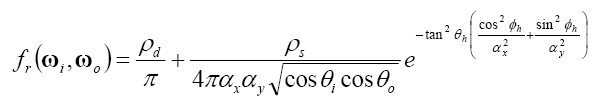
The Ward's BRDF is an elliptical Gaussian function [Ward92]:
However, this equation is not enough for an efficient implementation. First, we can separate the diffuse and specular components into 2 BSxF, and use Get BSDF to add them as 2 independent surface properties of the material. In this way the probability of (wi,wo) below will be closer to the BRDF. Also we pre-compute all constants in the BRDF, such as inverse ax and ay.
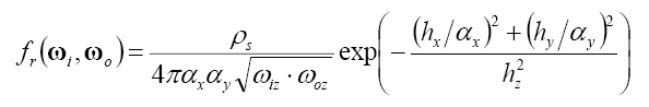
Second, in pbrt the input of function f() is wo and wi, and we can directly generate unnormalized h from them. If we re-arrange the BRDF equation, we can find that h is enough for evaluating the BRDF:
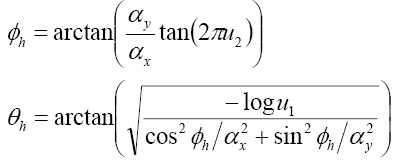
Now we examine the function Sampl_f(), which generates wi and pdf based on 2 random variables. Ward uses these random variables to obtain the polar and azimuthal angles of the half vector:
Note that the arctangent in the second equation in accidently omitted in the original paper [Walter05]. This method does not generate uniformly weighted sample as Ward claimed in the paper. If we use cosine-weighting, the result looks bad due to large variance.
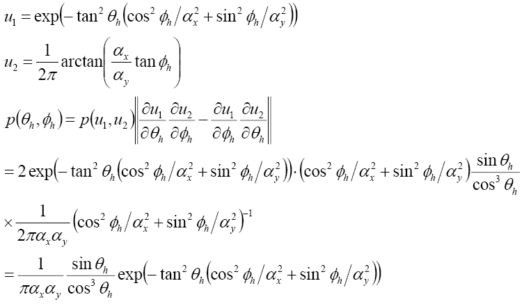
To solve this problem, we need to know the exact probability using this transformation. Since Ward did not provide the transformation, we do it in backward:
We then transform this pdf into the solid angle form and then transform it into a function of wi. These two steps are derived in the textbook for other BRDFs and thus we skip them here. The resulting pdf is
We can see it is closer to the BRDF and therefore the sampling will be more efficient. This result is presented in [Walter05] but the derivation is omitted.
The program can be made more efficient if we combin f(), sample_f(), and Pdf() into a single function because there are some repetitive routines. However we don't do that alot because we want to preserve the original structure of the program. The only trick we made is to pass the half vector h from sample_f() to f().
Result
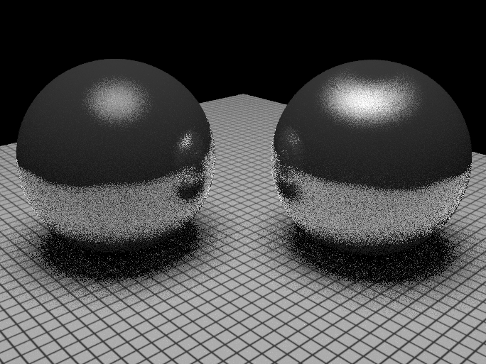
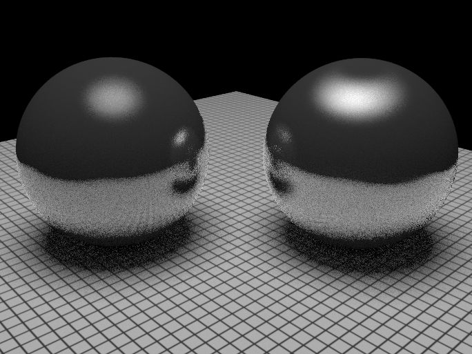
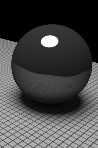
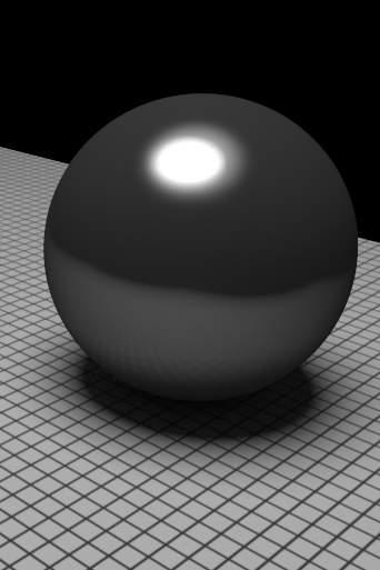
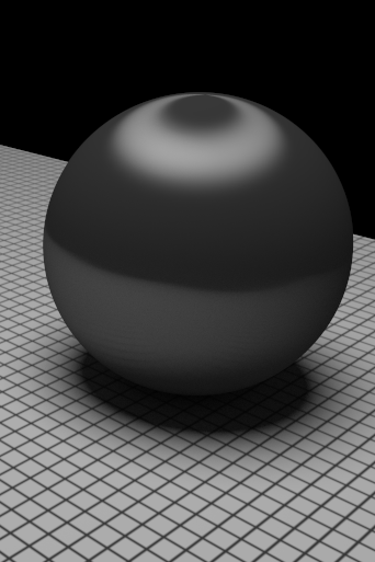
First we show the efficiency of the derived pdf, compared with simple cosine-sample the hemisphere (The separation of the diffusion and the specular components also significantly reduces the variance, which is not presented here). You can see the full-sized images by clicking them.
Cosine sampled pdf Exact pdf As you can see, the wrong pdf makes the results noisier, and overemphasizes the specularity.
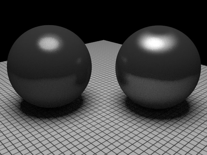
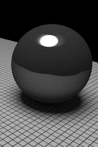
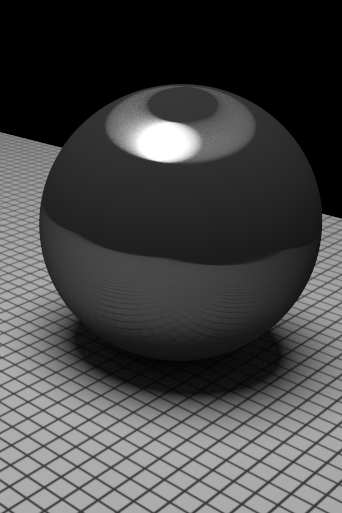
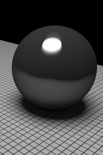
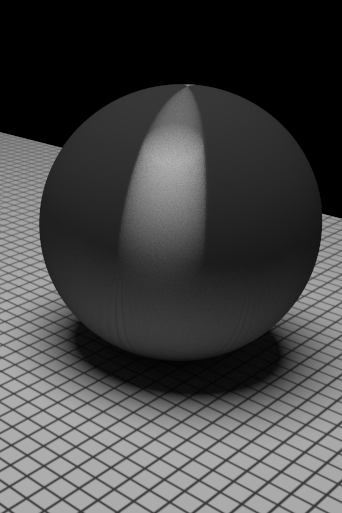
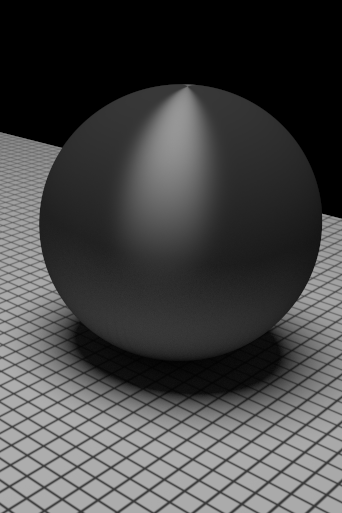
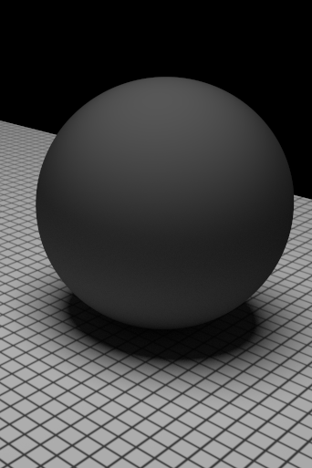
Finally we show the anisotropism of the Ward's BRDF. The images below are generated using 512 samples/pixel.

Downloads
Source code: ward.cpp (Put in src/materials)
MS .NET project: ward.vcproj (Put in src/win32/Projects)
Example scene using Ward's BRDF: spheres-ward.pbrt
References
- Ward, G. J. 1992. Measuring and modeling anisotropic reflection. In Proceedings of the 19th Annual Conference on Computer Graphics and interactive Techniques J. J. Thomas, Ed. SIGGRAPH '92. ACM Press, New York, NY, 265-272.
- Walter, B. Notes on the Ward BRDF. Technical report PCG-05-06, Program of Computer Graphics, Cornell University, April 2005.